Scanning SQUID microscopy
One of the original motivations for SuperScreen was to model scanning superconducting quantum interference device (SQUID) magnetometers/susceptometers used in scanning SQUID microscopy. In this notebook we demonstrate how SuperScreen can be used to calculate the mutual inductance between the field coil and pickup loop in state-of-the-art scanning SQUID susceptometers (Rev. Sci. Instrum. 87, 093702
(2016), arXiv:1605.09483).
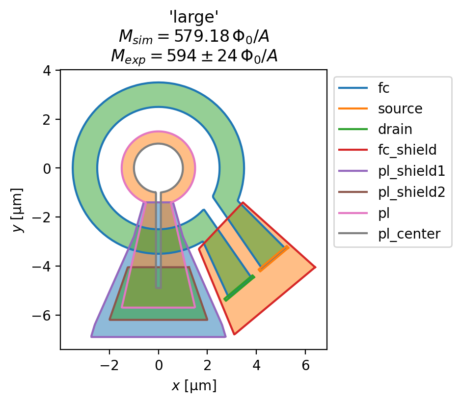
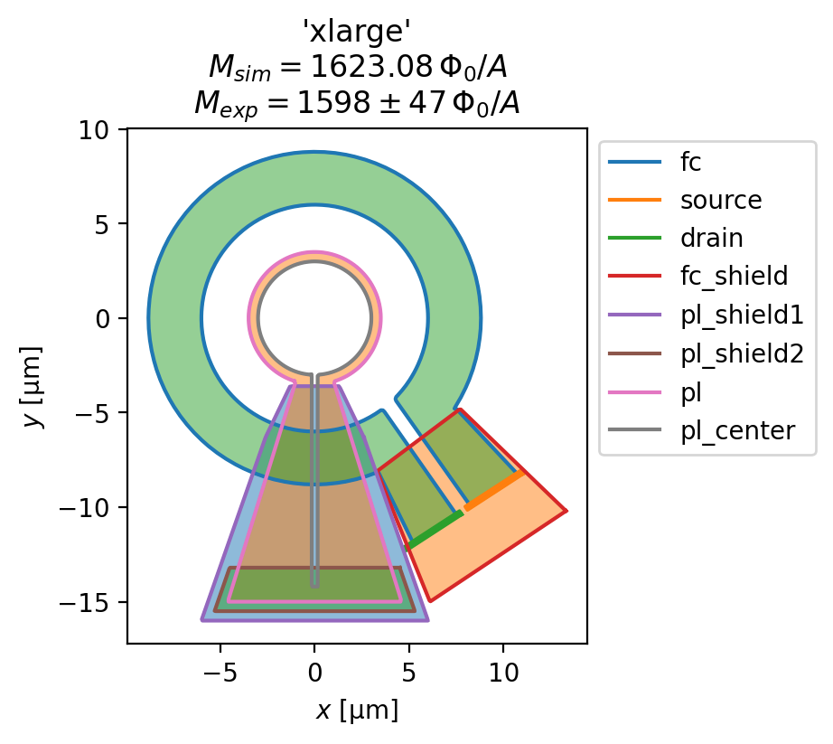
The layouts for four designs of scannning SQUID susceptometer are shown below (taken from Figure 4 of Kirtley, et al., Scanning SQUID susceptometers with sub-micron spatial resolution, Rev. Sci. Instrum. 87, 093702 (2016)).
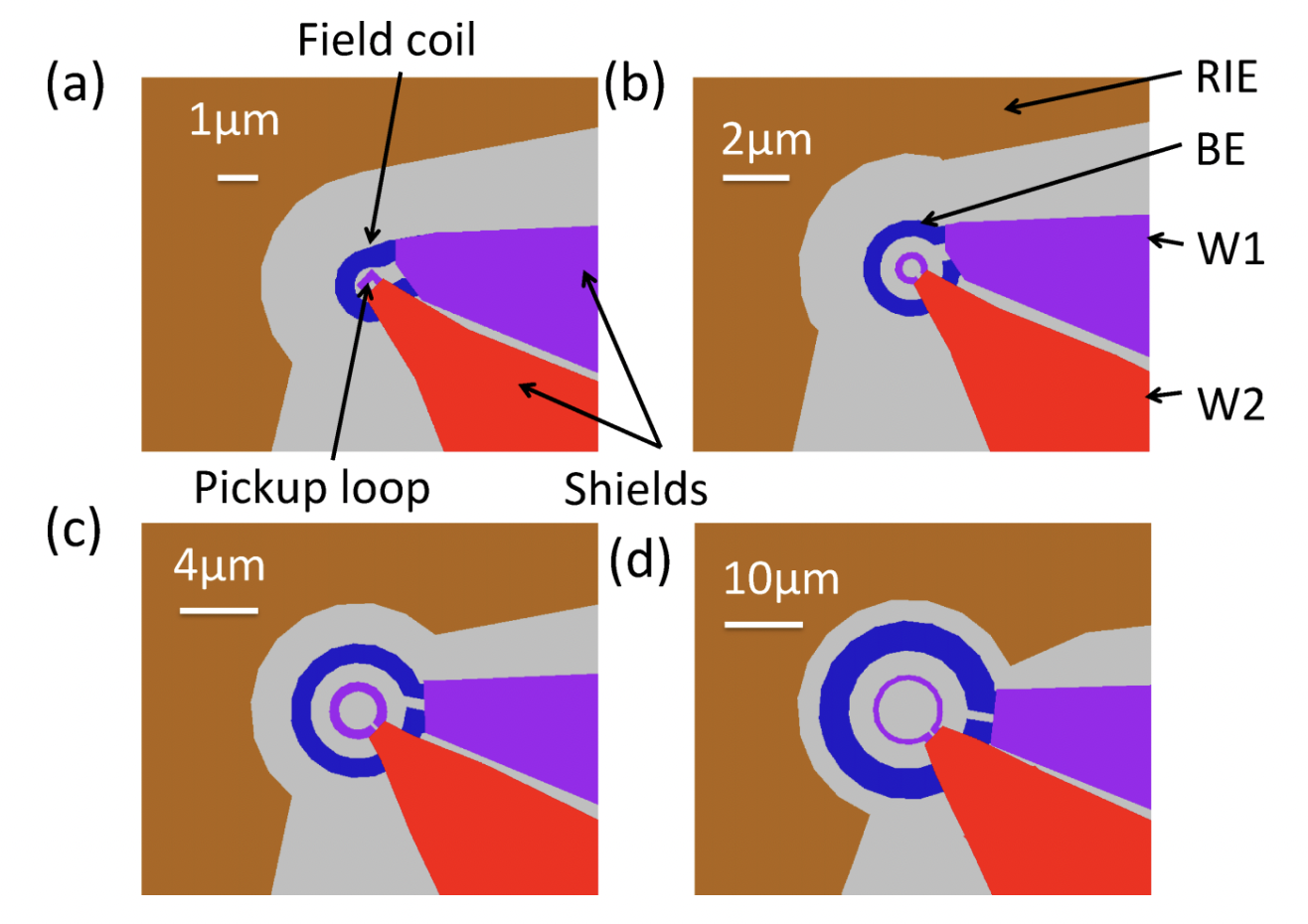
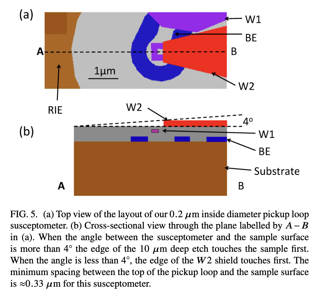
There are three relevant superconducting wiring layers, labeled “BE” (blue), “W1” (purple), and “W2” (red). The pickup loop, the flux-sennsing loop that is part of the SQUID circuit, sits in the purple “W1” wiring layer. The pickup loop is partially covered by a superconducting shield in the red “W2” wiring layer, which sits between the pickup loop and the sample being measured. A single-turn field coil sitting in the blue “BE” wiring layer can be used to locally apply a magnetic field to the sample. The layer structure of the SQUID susceptometers is shown below (taken from Figure 5 of Kirtley, et al., Scanning SQUID susceptometers with sub-micron spatial resolution, Rev. Sci. Instrum. 87, 093702 (2016)).
The pickup loop and field coil can be used to perform a mutual inductance AC susceptibility measurement in a reflection geometry. The presence of a paramagnetic or diamagnetic sample near the pickup loop and field coil modifies the mutual inductance between the two loops, and the strength of the modification is a measure of the magnetic susceptibility of the sample. Quantitative modeling of the magnetic response of such multi-layer superconducting circuits is important both for interpreting measurements and for designing next-generation sensors.
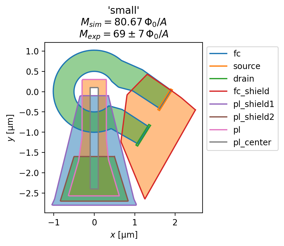
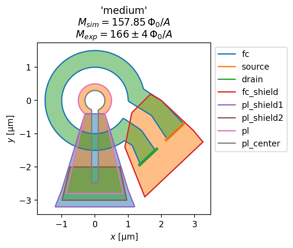
The experimentally measured values of the pickup loop - field coil mutual inductance (in units of \(\Phi_0/\mathrm{A}\), the flux induced in the pickup loop per unit current flowing in the field coil) are shown below. The value are taken from Table 1 of Rev. Sci. Instrum. 87, 093702 (2016). As shown below, we find excellent agreement between SuperScreen models derived from the
as-designed SQUID layouts and the experimentally measured mutual inductance.
[1]:
exp_mutuals = {
    "small": (69, 7),  # panel (a) in the first figure
    "medium": (166, 4),  # panel (b)
    "large": (594, 24),  # panel (c)
    "xlarge": (1598, 47),  # panel (d)
}
[2]:
# Automatically install superscreen from GitHub only if running in Google Colab
if "google.colab" in str(get_ipython()):
    %pip install --quiet git+https://github.com/loganbvh/superscreen.git
[3]:
%config InlineBackend.figure_formats = {"retina", "png"}
%matplotlib inline

import os
import sys

os.environ["OPENBLAS_NUM_THREADS"] = "1"

import matplotlib.pyplot as plt

plt.rcParams["figure.figsize"] = (5, 4)
plt.rcParams["font.size"] = 10

import superscreen as sc
from superscreen.geometry import box

sys.path.insert(0, "..")
import squids
[4]:
sc.version_table()
[4]:
| Software | Version |
|---|---|
| SuperScreen | 0.13.0 |
| Numpy | 2.4.4 |
| Numba | 0.65.1 |
| SciPy | 1.17.1 |
| matplotlib | 3.10.9 |
| IPython | 9.13.0 |
| Python | 3.12.12 (main, Apr 27 2026, 17:32:11) [GCC 11.4.0] |
| OS | posix [linux] |
| Number of CPUs | Physical: 1, Logical: 2 |
| BLAS Info | Generic |
| Sat May 02 11:59:53 2026 UTC | |
Define and solve the models
[5]:
squid_funcs = {
    "small": squids.ibm.small.make_squid,
    "medium": squids.ibm.medium.make_squid,
    "large": squids.ibm.large.make_squid,
    "xlarge": squids.ibm.xlarge.make_squid,
}
mesh_kwargs = {
    "small": dict(max_edge_length=0.1),
    "medium": dict(max_edge_length=0.1),
    "large": dict(max_edge_length=0.15),
    "xlarge": dict(max_edge_length=0.3),
}
Here, we simulate the reponse of the four SQUID susceptometers to a fixed current of 1 mA flowing counterclockwise in the field coil.
[6]:
solutions = {}
I_fc = "1 mA"
for name, make_squid in squid_funcs.items():
    squid = make_squid()
    squid.make_mesh(**mesh_kwargs[name])
    solutions[name] = sc.solve(
        squid,
        terminal_currents={"fc": {"source": I_fc, "drain": f"-{I_fc}"}},
        iterations=5,
        progress_bar=False,
    )[-1]
Evaluate the pickup loop - field coil mutual inductance
[7]:
for name, solution in solutions.items():
    squid = solution.device
    fig, ax = squid.draw()
    _ = squid.plot_polygons(ax=ax, legend=True)

    fluxoid = sum(solution.hole_fluxoid("pl_center"))
    mutual_inductance = (fluxoid / sc.ureg(I_fc)).to("Phi_0 / A").magnitude
    mean, rng = exp_mutuals[name]
    title = [
        f"{name!r}",
        rf"$M_{{sim}}={{{mutual_inductance:.2f}}}\,\Phi_0/A$",
        rf"$M_{{exp}}={{{mean}}}\pm{{{rng}}}\,\Phi_0/A$"
    ]
    ax.set_title("\n".join(title))
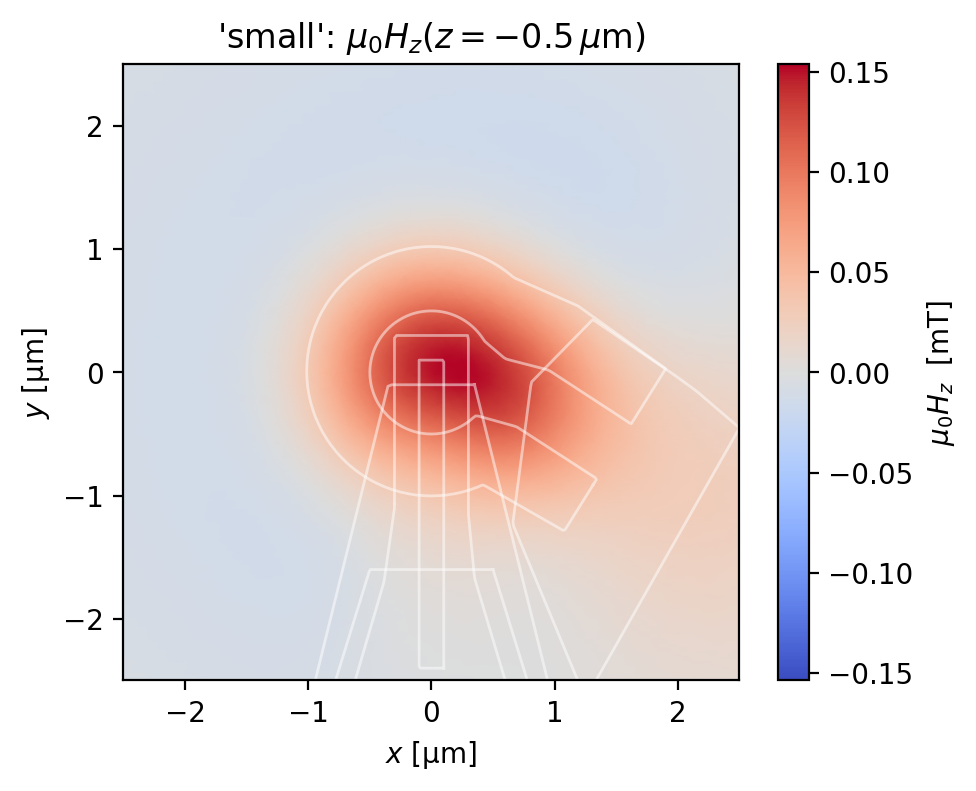
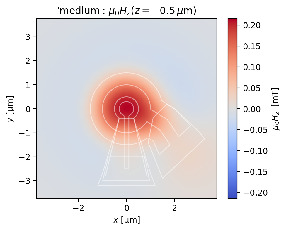
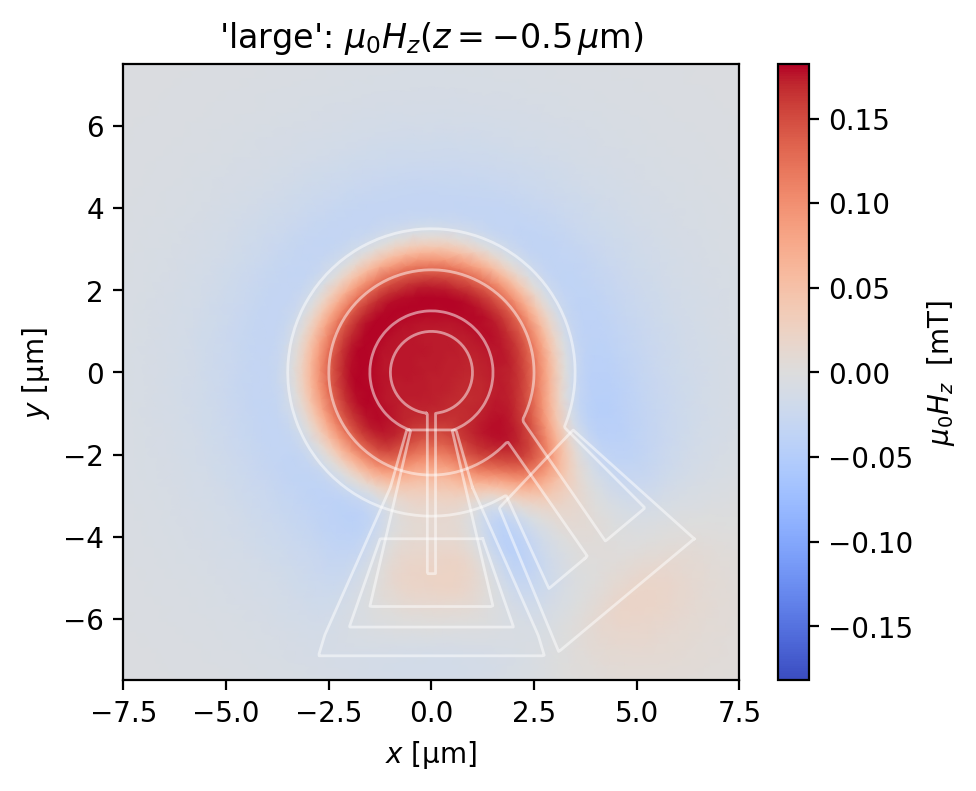
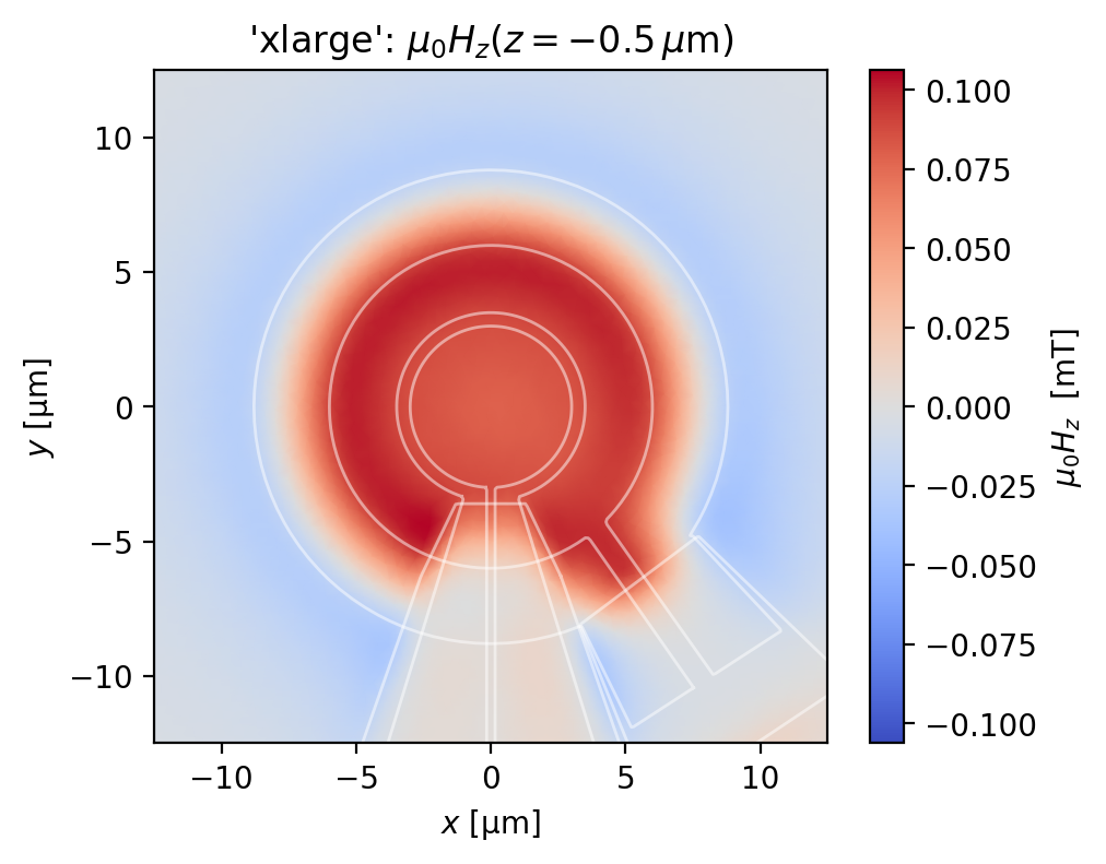
Evaluate the magnetic field generated by the susceptometer
Below, we plot the \(z\)-component of the magnetic field generated by the SQUID susceptometer field coil, evaluated at a plane 0.5 \(\mu\)m from the top wiring layer of the susceptometer.
[8]:
eval_regions = {
    # name: (width, height, z-position)
    "small": (5, 5, -0.5),
    "medium": (7.5, 7.5, -0.5),
    "large": (15, 15, -0.5),
    "xlarge": (25, 25, -0.5),
}
for name, solution in solutions.items():
    width, height, z = eval_regions[name]
    eval_mesh = sc.Polygon(points=box(width, height, points=201)).make_mesh(min_points=4000)
    fig, ax = solution.plot_field_at_positions(
        eval_mesh,
        zs=z,
        symmetric_color_scale=True,
        cmap="coolwarm",
    )
    squid = solution.device
    for polygon in squid.get_polygons(include_terminals=False):
        polygon.plot(ax=ax, color="w", lw=1, alpha=0.5)
    ax.set_title(rf"{name!r}: $\mu_0H_z(z={{{z}}}\,\mu\mathrm{{m}})$")
[ ]: