Working with polygons
At the core of each SuperScreen simulation is an instance of the superscreen.Device class, which represents the superconducting structure to be modeled. A Device is composed of one or more Layers that each lie in a plane parallel to the \(x-y\) plane (at position layer.z0) and have a specified penetration depth \(\Lambda\). Each layer contains one or more superconducting films, and each film contains zero or more holes. Films and holes are
represented by instances of the superscreen.Polygon class, which defines a 2D polygonal region.
[1]:
# Automatically install superscreen from GitHub only if running in Google Colab
if "google.colab" in str(get_ipython()):
    %pip install --quiet git+https://github.com/loganbvh/superscreen.git
[2]:
%config InlineBackend.figure_formats = {"retina", "png"}
%matplotlib inline

import os

os.environ["OPENBLAS_NUM_THREADS"] = "1"

import numpy as np
import matplotlib.pyplot as plt

plt.rcParams["figure.figsize"] = (4, 4)
plt.rcParams["font.size"] = 10

import superscreen as sc
[3]:
sc.version_table()
[3]:
| Software | Version |
|---|---|
| SuperScreen | 0.13.0 |
| Numpy | 2.4.4 |
| Numba | 0.65.1 |
| SciPy | 1.17.1 |
| matplotlib | 3.10.9 |
| IPython | 9.13.0 |
| Python | 3.12.12 (main, Apr 27 2026, 17:32:11) [GCC 11.4.0] |
| OS | posix [linux] |
| Number of CPUs | Physical: 1, Logical: 2 |
| BLAS Info | Generic |
| Sat May 02 11:58:32 2026 UTC | |
A Polygon is defined by a collection of (x, y) coordinates specifying its vertices; the vertices are stored as an n x 2 numpy.ndarray called polygon.points.
[4]:
# Define the initial geometry: a rectangular box specified as an np.ndarray
width, height = 10, 2
points = sc.geometry.box(width, height)
print(f"type(points) = {type(points)}, points.shape = {points.shape}")
type(points) = <class 'numpy.ndarray'>, points.shape = (100, 2)
[5]:
# Create a Polygon representing a "horizontal bar", hbar
hbar = sc.Polygon(points=points)
hbar.polygon
[5]:

The object passed to sc.Polygon(points=...) can be of any of the following:
An
n x 2array-like object, for example annp.ndarrayor a list of(x, y)coordinatesAn existing
sc.Polygoninstance (in which case, the new object will be a copy of the existing one)An instance of LineString, LinearRing, or Polygon from the shapely package
[6]:
(
    sc.Polygon(points=hbar.points)
    == sc.Polygon(points=hbar.polygon)
    == sc.Polygon(points=hbar)
    == hbar.copy()
    == hbar
)
[6]:
True
Every instance of sc.Polygon has a property, instance.polygon, which returns a corresponding shapely Polygon object. Among other things, this is usefuly for quickly visualizing polygons.
There are several methods for transforming the geometry of a single Polygon:
polygon.translate(dx=0, dy=0)polygon.rotate(degrees, origin=(0, 0))polygon.scale(xfact=1, yfact=1, origin=(0, 0))polygon.buffer(distance, ...)
There are also three methods for combining multiple Polygon-like objects:
polygon.union(*others): logical union ofpolygonwith each object in the iterableothersSee also:
sc.Polygon.from_union([...])polygon.intersection(*others): logical intersection ofpolygonwith each object in the iterableothersSee also:
sc.Polygon.from_intersection([...])polygon.difference(*others): logical difference ofpolygonwith each object in the iterableothersSee also:
sc.Polygon.from_difference([...])
Note that the elements of the iterable others can be of any type that can be passed in to sc.Polygon(points=...) (see above).
[7]:
# Copy hbar and rotate the copy 90 degrees counterclockwise
vbar = hbar.rotate(90)
vbar.polygon
[7]:

[8]:
# Create a new Polygon that is the union of hbar and vbar: "+"
plus = hbar.union(vbar)
# # The above is equivalent to either of the following:
# plus = vbar.union(hbar)
# plus = sc.Polygon.from_union([hbar, vbar])
plus.polygon
[8]:

[9]:
# Rotate the "+" by 45 degrees to make an "X"
X = plus.rotate(45)
X.polygon
[9]:

[10]:
# Create a new polygon with all edges offset (eroded) by a distance of -0.5
thinX = X.buffer(-0.5)
thinX.polygon
[10]:

[11]:
# Create a new polygon with all edges offset (expanded) by a distance of 0.5
thickX = X.buffer(0.5)
thickX.polygon
[11]:

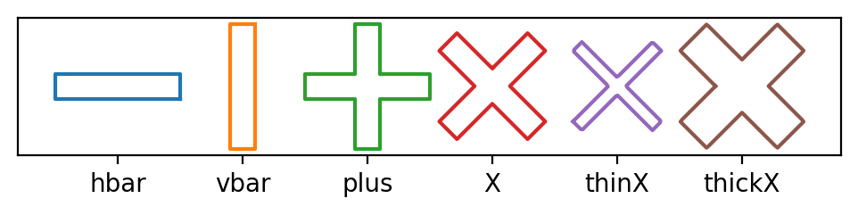
[12]:
polygons = [hbar, vbar, plus, X, thinX, thickX]
labels = ["hbar", "vbar", "plus", "X", "thinX", "thickX"]

fig, ax = plt.subplots(figsize=(6, 1))

for i, polygon in enumerate(polygons):
    polygon.translate(dx=width * i).plot(ax=ax)

ax.set_xticks([width * i for i, _ in enumerate(labels)])
ax.set_xticklabels(labels)
_ = ax.set_yticks([])
[13]:
X.union(plus).polygon
[13]:

[14]:
X.intersection(plus).polygon
[14]:

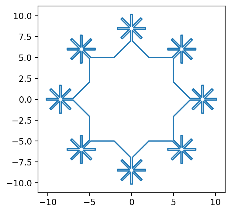
Using the methods demonstrated above, intricate geometries can be constructed from simple building blocks in just a few lines of code.
[15]:
size = 10

hbar = sc.Polygon(points=sc.geometry.box(size / 3, size / 50))
plus = hbar.union(hbar.rotate(90))
star = plus.union(plus.rotate(45))

star_dx = 1.2 * size * np.sqrt(2) / 2

snowflake = (
    sc.Polygon(points=sc.geometry.box(size, size))
    .rotate(45)
    .union(
        *(star.translate(dx=star_dx).rotate(degrees) for degrees in [0, 90, 180, 270])
    )
)
snowflake = snowflake.union(snowflake.rotate(45))
[16]:
ax = snowflake.plot()
[17]:
print(f"Polygon area: snowflake.area = {snowflake.area:.3f}")
print(f"Polygon width and height: snowflake.extents = {snowflake.extents}")
Polygon area: snowflake.area = 136.622
Polygon width and height: snowflake.extents = (20.303896081810475, 20.303896081810475)
In SuperScreen, all polygons must be simply-connected, i.e. have no holes.
[18]:
circle = sc.Polygon(points=sc.geometry.circle(10))
hole = circle.scale(0.5, 0.5)
try:
    ring = circle.difference(hole)
except ValueError as e:
    print(f"ValueError('{e}')")
ValueError('Expected a simply-connected polygon.')
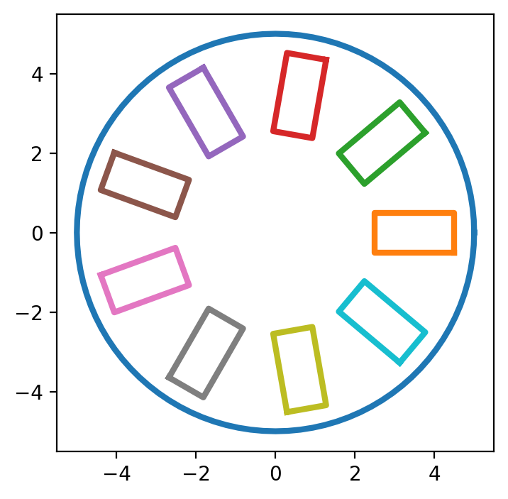
However, SuperScreen does allow you to model multiply-connected films. A film with \(h\) holes in it is modeled as \(h + 1\) separate sc.Polygon objects:
[19]:
h = 9
circle = sc.Polygon(points=sc.geometry.circle(5))
holes = [
    sc.Polygon(points=sc.geometry.box(2, 1)).translate(3.5).rotate(theta)
    for theta in np.linspace(0, 360, h, endpoint=False)
]

ax = circle.plot(lw=3)
for hole in holes:
    hole.plot(ax=ax, lw=3)
    # Boolean array indicating whether each point in hole.points
    # lies within the circle
    points_in_circle = circle.contains_points(hole.points)
    assert isinstance(points_in_circle, np.ndarray)
    assert points_in_circle.shape[0] == hole.points.shape[0]
    assert points_in_circle.dtype == np.dtype(bool)
    assert points_in_circle.all()

    # Alternatively, use shapely to check whehther the hole's polygon
    # lies within the circle's polygon
    assert circle.polygon.contains(hole.polygon)
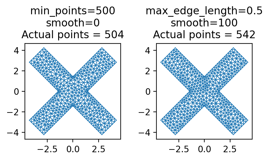
Meshing Polygons
Individual polygons can be meshed using the Polygon.make_mesh() method.
[20]:
setups = [
    dict(min_points=500, smooth=0),
    dict(max_edge_length=0.5, smooth=100),
]

fig, axes = plt.subplots(1, len(setups), figsize=(2 * (len(setups) + 0.5), 2))

for ax, options in zip(axes, setups):
    # Generate a mesh with the specified options
    mesh = X.make_mesh(**options)

    # Plot the mesh
    ax.set_aspect("equal")
    title = [f"{key}={value!r}" for key, value in options.items()]
    title.append(f"Actual points = {len(mesh.sites)}")
    ax.triplot(mesh.sites[:, 0], mesh.sites[:, 1], mesh.elements, linewidth=0.75)
    ax.set_title("\n".join(title))
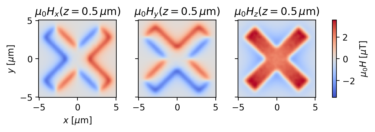
This can come in handy if, for example, you want to use a Polygon to define an applied magnetic field rather than include it in a Device to solve.
Here we calculate the vector magnetic field from a magnetic “X” lying in the \(x-y\) plane with uniform out-of-plane magnetization. We’ll assume that the dimensions of the “X” are in microns and that its magnetization (area density of magnetic moments) is \(\vec{m}=1\,\mu_\mathrm{B}/\mathrm{nm}^2\,\hat{z}\), where \(\mu_\mathrm{B}\) is the Bohr magneton.
[21]:
# Generate the mesh
mesh = X.make_mesh(min_points=1000)
x, y = mesh.sites[:, 0], mesh.sites[:, 1]

# (x, y, z) position of each vertex
vertex_positions = np.stack([x, y, np.zeros_like(x)], axis=1)

# Calculate the effective area of each vertex in the mesh
vertex_areas = mesh.vertex_areas * sc.ureg("um ** 2")

# Define the magnetic moment of each mesh vertex
z_hat = np.array([0, 0, 1])  # unit vector in the z direction
magnetization = sc.ureg("1 mu_B / nm ** 2")
vertex_moments = z_hat * magnetization * vertex_areas[:, np.newaxis]
# Convert to units of Bohr magnetons
vertex_moments = vertex_moments.to("mu_B").magnitude
The function superscreen.sources.DipoleField returns a superscreen.Parameter that calulates the magnetic field (in Tesla) from a disribution of magnetic dipoles.
[22]:
field_param = sc.sources.DipoleField(
    dipole_positions=vertex_positions,
    dipole_moments=vertex_moments,
)
Evaluate the magnetic field from the “X”:
[23]:
# Coordinates at which to evaluate the magnetic field (in microns)
N = 101
eval_xs = eval_ys = np.linspace(-5, 5, N)
eval_z = 0.5
xgrid, ygrid, zgrid = np.meshgrid(eval_xs, eval_ys, eval_z)
xgrid = np.squeeze(xgrid)
ygrid = np.squeeze(ygrid)
zgrid = np.squeeze(zgrid)

# field_param returns shape (N * N, 3), where the last axis is field component
# and the units are Tesla
field = field_param(xgrid.ravel(), ygrid.ravel(), zgrid.ravel()) * sc.ureg("tesla")
# Reshape to (N, N, 3), where the last axis is field component,
# and convert to microTesla
field = field.reshape((N, N, 3)).to("microtesla").magnitude
Plot the results:
[24]:
fig, axes = plt.subplots(
    1, 3, figsize=(6, 2), sharex=True, sharey=True, constrained_layout=True
)

vmax = max(abs(field.min()), abs(field.max()))
vmin = -vmax
kwargs = dict(vmin=vmin, vmax=vmax, shading="auto", cmap="coolwarm")

for i, (ax, label) in enumerate(zip(axes, "xyz")):
    ax.set_aspect("equal")
    im = ax.pcolormesh(xgrid, ygrid, field[..., i], **kwargs)
    ax.set_title(f"$\\mu_0H_{{{label}}}(z={{{eval_z}}}\\,\\mu\\mathrm{{m}})$")
cbar = fig.colorbar(im, ax=axes)
cbar.set_label("$\\mu_0H$ [$\\mu$T]")
_ = axes[0].set_xlabel("$x$ [$\\mu$m]")
_ = axes[0].set_ylabel("$y$ [$\\mu$m]")
[ ]: