Background
The goal of SuperScreen is to model the magnetic response of a thin superconducting film,
or a structure composed of multiple superconducting films (which may or may not lie in the same plane),
to an applied inhomogeneous out-of-plane magnetic field
\(H_{z,\,\mathrm{applied}}(x, y, z)\).
Given \(H_{z,\,\mathrm{applied}}(x, y, z)\) and information about the geometry and magnetic penetration depth of all films in a superconducting structure, we aim to calculate the thickness-integrated current density \(\vec{J}(x, y)\) at all points inside the films, from which one can calculate the vector magnetic field \(\vec{H}(x, y, z)\) at all points both inside and outside the films.
Brandt’s Method
A convenient method for solving this problem was introduced in [Brandt-PRB-2005], and used in [Kirtley-RSI-2016] and [Kirtley-SST-2016] to model the magnetic response of scanning Superconducting Quantum Interference Device (SQUID) susceptometers.
Model
In the London model of superconductivity, the magnetic field \(\vec{H}(\vec{r})\) and 3D current density \(\vec{j}(\vec{r})\) in a superconductor with London penetration depth \(\lambda\) obey the second London equation: \(\nabla\times\vec{j}(\vec{r})=-\vec{H}(\vec{r})/\lambda^2\), where \(\nabla=\left(\frac{\partial}{\partial x}, \frac{\partial}{\partial y}, \frac{\partial}{\partial z}\right)\).
Brandt’s model assumes that the current density \(\vec{j}\) is approximately independent of \(z\), such \(\vec{j}(x, y, z)\approx\vec{j}_{z_0}(x, y)\) for a film lying parallel to the \(x-y\) plane at vertical position \(z_0\). Working now with the thickness-integrated current density (or “sheet current”) \(\vec{J}(x, y)=\vec{j}_{z_0}(x, y)\cdot d\), where \(d\) is the thickness of the film, the second London equation reduces to
where \(\Lambda=\lambda^2/d\) is the effective penetration depth of the superconducting film (equal to half the Pearl length [Pearl-APL-1964]).
Note
The assumption \(\vec{j}(x, y, z)\approx\vec{j}_{z_0}(x, y)\) is valid for films that are much thinner than their London penetration depth (i.e. \(d\ll\lambda\)), such that \(\Lambda=\lambda^2/d\gg\lambda\). However the model has been applied with some success in structures with \(\lambda\lesssim d\) [Kirtley-RSI-2016] [Kirtley-SST-2016]. Aside from this limitation, the method described below can in principle to used to model films with any effective penetration depth \(0\leq\Lambda<\infty\).
Because the sheet current has zero divergence in the superconducting film (\(\nabla\cdot\vec{J}=0\)) except at small contacts where current can be injected, one can express the sheet current in terms of a scalar potential \(g(x, y)\), called the stream function:
The stream function \(g\) can be thought of as the local magnetization of the film, or the area density of tiny dipole sources. We can re-write Eq. 1 for a 2D film in terms of \(g\):
where \(\nabla^2=\nabla\cdot\nabla\) is the Laplace operator. (The last line follows from the fact that \(\nabla\cdot\left(g(x,y)\hat{z}\right) = 0\)). From Ampere’s Law, the \(z\)-component of the magnetic field at position \(\vec{r}=(x, y, z)\) due to a sheet of current lying in the \(x-y\) plane (at height \(z'\)) with stream function \(g(x', y')\) are given by:
\(H_{z,\,\mathrm{applied}}(\vec{r})\) is an externally-applied magnetic field (which we assume to have no \(x\) or \(y\) component), \(S\) is the film area (with \(g = 0\) outside of the film), and \(Q_z(\vec{r},\vec{r}')\) is a dipole kernel function which gives \(z\)-component of the magnetic field at position \(\vec{r}=(x, y, z)\) due to a dipole of unit strength at poition \(\vec{r}'=(x', y', z')\):
where \(\Delta z = z - z'\) and \(\rho=\sqrt{(x-x')^2 + (y-y')^2}\). Comparing Eq. 3 and Eq. 4, we have in the plane of the film:
(where now \(\vec{r}\) and \(\vec{r}'\) are 2D vectors, i.e. \(\Delta z=0\), since the film is in the same plane as itself). From Eq. 6, we arrive at an integral equation relating the stream function \(g\) for points inside the superconductor to the applied field \(H_{z,\,\mathrm{applied}}\):
The goal, then, is to solve (invert) Eq. 7 for a given \(H_{z,\,\mathrm{applied}}\) and film geometry \(S\) to obtain \(g\) for all points inside the film (with \(g=0\) enforced outside the film). Once \(g(\vec{r})\) is known, full vector magnetic field \(\vec{H}\) can be calculated at any point \(\vec{r}\) using Eq. 2 and the Biot-Savart law.
Films with holes
In films that have holes (regions of vacuum completely surrounded by superconductor), each hole \(k\) can contain a trapped flux \(\Phi_k\), with an associated circulating current \(I_{\mathrm{circ},\,k}\). The (hypothetical) applied field that would cause such a circulating current is given by Eq. 7 if we set \(g(\vec{r})=I_{\mathrm{circ},\,k}\) for all points \(\vec{r}\) lying inside hole \(k\):
In this case, we modify the left-hand side of Eq. 7 as follows:
Structures with multiple films
The magnetic response of structures composed of multiple films can be found self-consistently using an iterative approach. Each film \(F\) exists in a layer \(\ell\) lying in the plane \(z=z_F=z_\ell\), and a single layer can contain multiple non-overlapping films. The stream functions and fields for all films can be computed self-consistently using the following recipe:
Calculate the stream function \(g_F(\vec{r})\) for each film \(F\) by solving Eq. 9 given an applied field \(H_{z,\,\mathrm{applied}}(\vec{r}, z_F)\).
For each film \(F\), calculate the \(z\)-component of the field due to the currents in all other films \(k\neq F\) using Eq. 2 and the Biot-Savart law.
Re-solve Eq. 9 taking the new applied field for each film to be the original applied field plus the sum of screening fields from all other films. This is accomplished by setting:
\[H_{z,\,\mathrm{applied}}(\vec{r}, z_F) \leftarrow H_{z,\,\mathrm{applied}}(\vec{r}, z_F) + \sum_{k\neq F} \int_S Q_z(\vec{r},\vec{r}')g_k(\vec{r}')\,\mathrm{d}^2r'.\]Repeat steps 1-3 until the stream functions and fields converge.
Applied bias currents
A bias current can be applied to a given film through one or more terminals or current contacts. See Terminal currents for more details.
Finite Element Implementation
Here we describe the numerical implementation of the model outlined above.
Discretized model
In order to numerically solve Eq. 4 and Eq. 9, we have to discretize the films, holes, and the vacuum regions surrounding them. We use a triangular (Delaunay) mesh, consisting of \(n\) points (or vertices) which together form \(m\) triangles.
Below we denote column vectors and matrices using bold font. \(\mathbf{A}\mathbf{B}\) denotes matrix multiplication, with \((\mathbf{A}\mathbf{B})_{ij}=\sum_{k=1}^\ell A_{ik}B_{kj}\) (\(\ell\) being the number of columns in \(\mathbf{A}\) and the number of rows in \(\mathbf{B}\)). Column vectors are treated as matrices with \(\ell\) rows and \(1\) column. On the other hand, we denote element-wise multiplication with a lower dot: \((\mathbf{A}.\mathbf{B})_{ij}=A_{ij}B_{ij}\). \(\mathbf{A}^T\) denotes the transpose of matrix \(\mathbf{A}\).
The matrix version of Eq. 4 is:
The \(n\times n\) kernel matrix \(\mathbf{Q}\) represents the kernel function \(Q_z(\vec{r},\vec{r}')\) for all points lying in the plane of the film, and the \(n\times 1\) weight vector \(\mathbf{w}\), which assigns an effective area to each vertex in the mesh, represents the differential element \(\mathrm{d}^2r'\). Both \(\mathbf{Q}\) and \(\mathbf{w}\) are solely determined by the geometry of the mesh, so they only need to be computed once for a given device. \(\mathbf{h}_z\), \(\mathbf{h}_{z,\,\mathrm{applied}}\), and \(\mathbf{g}\) are all \(n\times 1\) vectors, with each row representing the value of the quantity at the corresponding vertex in the mesh. The vector \(\mathbf{w}\) is equal to the diagonal of the “lumped mass matrix” \(\mathbf{M}\): \(w_i=M_{ii} = \frac{1}{3}\sum_{t\in\mathcal{N}(i)}\mathrm{area}(t)\), where \(\mathcal{N}(i)\) is the set of triangles \(t\) adjacent to vertex \(i\). The kernel matrix \(\mathbf{Q}\) is defined in terms of a matrix with \((\mathbf{q})_{ij} = \left(4\pi|\vec{r}_i-\vec{r}_j|^3\right)^{-1}\) (which is \(\lim_{\Delta z\to 0}Q_z(\vec{r},\vec{r}')\) cf. Eq. 5), and a vector \(\mathbf{C}\):
where \(\delta_{ij}\) is the Kronecker delta function. The diagonal terms involving \(\mathbf{C}\) are meant to work around the fact that \((\mathbf{q})_{ii}\) diverge (see [Brandt-PRB-2005] for more details), and the vector is defined as
where \(\Delta x=(x_\mathrm{max}-x_\mathrm{min})/2\) and \(\Delta y=(y_\mathrm{max}-y_\mathrm{min})/2\) are half the side lengths of a rectangle bounding the modeled film(s) and \((\bar{x}, \bar{y})\) are the coordinates of the center of the rectangle. The matrix version of Eq. 9 is:
(where we exclude points in the mesh lying outside of the superconducting film, but keep points inside holes in the film). \(\mathbf{\nabla}^2\) is the Laplace operator, an \(n\times n\) matrix defined such that \(\mathbf{\nabla}^2\mathbf{f}\) computes the Laplacian \(\nabla^2f(x,y)\) of a function \(f(x,y)\) defined on the mesh.
Eq. 13 is a matrix equation relating the applied field to the stream function inside a superconducting film, which can efficiently be solved (e.g. by matrix inversion) for the unknown vector \(\mathbf{g}\), the stream function inside the film. Since the stream function outside the film and inside holes in the film is already known, solving Eq. 13 gives us the stream function for the full mesh. Defining \(\mathbf{K} = \left(\mathbf{Q}\cdot\mathbf{w}^T-\Lambda\mathbf{\nabla}^2\right)^{-1}\), we have
If there is a vortex containing flux \(\Phi_j\) trapped in a film at position \(\vec{r}_j\) indexed as mesh vertex \(j\), then for each position \(\vec{r}_i\) within that film, we add to the stream function \(g_i\) the quantity \(\mu_0^{-1}\Phi_jK_{ij} / w_{j}\), here \(K_{ij}\) is an element of the inverse matrix defined above, and \(w_{j}\) is an element of the weight matrix which assigns an effective area to the mesh vertex at which the vortex is located. This process amounts to numerically inverting Eq. 9 in the presence of delta-function magnetic sources representing trapped vortices, as described in [Brandt-PRB-2005].
Once the stream function \(\mathbf{g}\) is known for the full mesh, the sheet current flowing in the film can be computed from Eq. 2, the \(z\)-component of the total field at the plane of the film can be computed from Eq. 10, and the full vector magnetic field \(\vec{H}(x, y, z)\) at any point in space can be computed from Eq. 4 (and its analogs for the \(x\) and \(y\) components of the field).
Laplace and gradient operators
The definitions of the Laplace operator \(\mathbf{\nabla}^2\) (also called the Laplace-Beltrami operator) and the gradient operator \(\vec{\nabla}=(\nabla_x, \nabla_y)^T\) deserve special attention, as these two operators reduce the problem of solving a partial differential equation to the problem of solving a matrix equation [Laplacian-SGP-2014]. Given a mesh consisting of \(n\) vertices and \(m\) triangles, and a scalar field \(f(x, y)\) represented by an \(n\times 1\) vector \(\mathbf{f}\) containing the values of the field at the mesh vertices, the goal is to construct matrices \(\nabla^2\) and \(\vec{\nabla}=(\nabla_x, \nabla_y)^T\) such that the matrix products \(\nabla^2\mathbf{f}\) and \(\vec{\nabla}\mathbf{f}\) approximate the Laplacian \(\left(\frac{\partial^2f}{\partial x^2}+\frac{\partial^2f}{\partial y^2}\right)\) and the gradient \(\left(\frac{\partial f}{\partial x}, \frac{\partial f}{\partial y}\right)\) of \(f(x, y)\) at the mesh vertices.
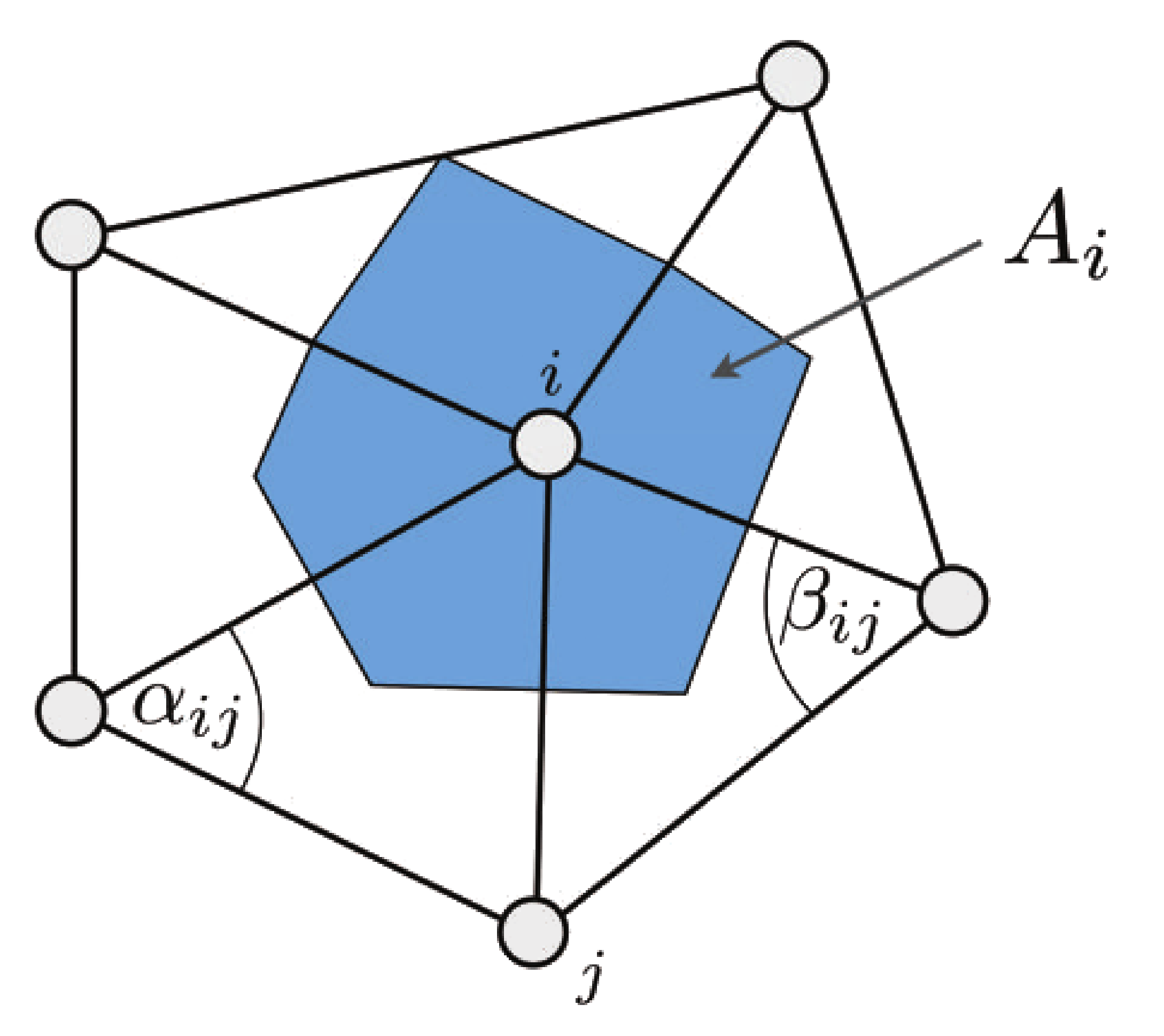
As described in [Vaillant-Laplacian-2013] and [Laplacian-SGP-2014] the Laplace operator \(\mathbf{\nabla}^2\) for a mesh is defined in terms of two matrices, the mass matrix \(\mathbf{M}\) and the Laplacian matrix \(\mathbf{L}\): \(\mathbf{\nabla}^2 = \mathbf{M}^{-1}\mathbf{L}\) The mass matrix gives an effective area to each vertex in the mesh. There are multiple ways to construct the mass matrix, but here we use a “lumped” mass matrix, which is diagonal with elements \((\mathbf{M})_{ii} = \sum_{t\in\mathcal{N}(i)}\frac{1}{3}\mathrm{area}(t)\), where \(\mathcal{N}(i)\) is the set of triangles \(t\) adjacent to vertex \(i\). (See image below, where \((\mathbf{M})_{ii} = A_i\). Image reference: [Vaillant-Laplacian-2013].) The vector \(\mathbf{w}\) discussed above is simply the diagonal of the mass matrix \(\mathbf{M}\).
The Laplacian matrix \(\mathbf{L}\) is defined in terms of the weight matrix \(\mathbf{W}\):
There are several different methods for constructing the weight matrix \(\mathbf{W}\):
Uniform weighting: In this case, \(\mathbf{W}\) is simply the adjacency matrix for the mesh.
\[\begin{split}W_{ij} = \begin{cases} 0&\text{if }i=j\\ 1&\text{if }i\text{ is adjacent to }j\\ 0&\text{otherwise} \end{cases}\end{split}\]Inverse-Euclidean weighting: Each edge is weighted by the inverse of its length: \(|\vec{r}_i-\vec{r}_j|^{-1}\), where \(\vec{r}_i\) is the position of vertex \(i\).
\[\begin{split}W_{ij} = \begin{cases} 0&\text{if }i=j\\ |\vec{r}_i-\vec{r}_j|^{-1}&\text{if }i\text{ is adjacent to }j\\ 0&\text{otherwise} \end{cases}\end{split}\]Half-cotangent weighting: Each edge is weighted by the half the sum of the cotangents of the two angles opposite to it. See image above. Image reference: [Vaillant-Laplacian-2013].).
\[\begin{split}W_{ij} = \begin{cases} 0&\text{if }i=j\\ \frac{1}{2}\left(\cot\alpha_{ij}+\cot\beta_{ij}\right)&\text{if }i\text{ is adjacent to }j\\ 0&\text{otherwise} \end{cases}\end{split}\]
Finally, the Laplace operator is given by:
By default, SuperScreen uses half-cotangent weighting.
We construct the two \(n\times n\) gradient matrices \(\nabla_x\) and \(\nabla_y\), using the “average gradient on a star” (or AGS) approach [Mancinelli-STAG-2019]. Briefly, we first construct two \(m\times n\) matrices, \(\vec{\nabla}_t=(\nabla_{t,x}, \nabla_{t,y})^T\) using “per-cell linear estimation” (or PCE) [Mancinelli-STAG-2019], where \(\nabla_{t,x}\mathbf{f}\) maps the field values at the vertices \(\mathbf{f}\) to an estimate of the \(x\)-component of the gradient at the triangle centroids (centers-of-mass). The matrices \(\nabla_x\) and \(\nabla_y\) are then computed by, for each vertex \(i\), taking the weighted average of \(\nabla_{t,x}\) and \(\nabla_{t,y}\) over adjacent triangles \(t\in\mathcal{N}(i)\), with weights given by the angle between the two sides of the triangle adjacent to the vertex. The resulting \(\vec{\nabla}=(\nabla_x, \nabla_y)^T\) is a \(2\times n\times n\) stack of matrices defined such that \(\vec{\nabla}\mathbf{f}\) produces a \(2\times n\) matrix representing the gradient of \(f(x, y)\) at the mesh vertices, with the first and second rows of \(\vec{\nabla}\mathbf{f}\) containing the \(x\) and \(y\) components of the gradient, respectively.
Inhomogeneous Films
The London equation (Eq. 1) is valid only under the assumption that the London penetration depth \(\lambda\), a proxy for the superfluid density, is constant as a function of position. In cases where the superfluid density varies as a function of position, Ginzburg-Landau theory provides a more accurate description of the magnetic response of the system. Nevertheless, in an effort to model inhomogeneous superconductors using London theory, one can write out the “inhomogeneous second London equation” for a superconductor with spatially-varying London penetration depth \(\lambda(\vec{r})\) ([Cave-Evetts-LTP-1986], [Kogan-Kirtley-PRB-2011]):
In the 2D limit, i.e. a thin film with thickness \(d\ll\lambda(x, y)\) lying parallel to the \(x-y\) plane carrying sheet current density \(\vec{J}(x, y)=\vec{j}(\vec{r})\cdot d\) we have:
where \(\Lambda=\Lambda(x, y)\), \(g=g(x, y)\), \(\vec{\nabla}=\left(\frac{\partial}{\partial x},\frac{\partial}{\partial y}\right)\), and \(\vec{J}=\vec{J}(x, y)=\vec{\nabla}\times(g\hat{z})\).
If one defines an inhomogeneous effective penetration depth \(\Lambda(x, y)\) in a SuperScreen model, Eq. 16, rather than Eq. 1, is solved numerically as follows. For a mesh with \(n\) vertices, the effective penetration depth is represented by an \(n\times 1\) vector \(\mathbf{\Lambda}\). Eq. 13 and Eq. 14 are updated according to:
The notation \(\vec{\nabla}\mathbf{f}\cdot\vec{\nabla}\) indicates an inner (dot) product over the two spatial dimensions, resulting in an \(n\times n\) matrix such that \((\vec{\nabla}\mathbf{f}\cdot\vec{\nabla})\mathbf{g}\) computes \((\vec{\nabla}f(x, y))\cdot(\vec{\nabla}g(x, y))\) (see Laplace and gradient operators).
Note that, unlike Eq. 1 in which \(\Lambda\) is assumed to be constant as a function of position \(\vec{r}\), solutions to Eq. 16 do not necessarily satisfy the fluxoid quantization condition \(\Phi^f_S=0\) for simply-connected superconducting regions \(S\) in which \(\vec{\nabla}\Lambda(\vec{r})\neq0\) , where